GeoHealth Mapping GIS Training
for Monitoring and Evaluation or
Strategic Information Officers and Data Analysts for HIV

3.5. Proximity Analysis: Buffers
Determining catchment areas or the geographic area covered by a facility or programs is important to support strategic planning of HIV programs. Understanding all of the intervention points within a defined geographic area allows program planners to improve allocative efficiency and reduce duplication of efforts.
Proximity analysis determines how many points of interest are within a given radius. This analysis is useful when planning for health facilities service areas or zones. For example, a program planner can determine the number of villages within a given distance from a health facility and use this information to define the service zone or catchment area. Conducting a proximity analysis also allows program planners to understand which villages fall outside of the service area and remain underserved. This section will demonstrate how to carryout proximity analysis using buffers. Buffers are polygons generated at a distance around a feature of interest.
3.5.1 Objectives
- Define DIC catchment areas using buffers
You will need the files for Section_3_5 to complete this module.
3.5.2 Launch QGIS and start a new project
In this exercise we shall define catchment areas using buffers.
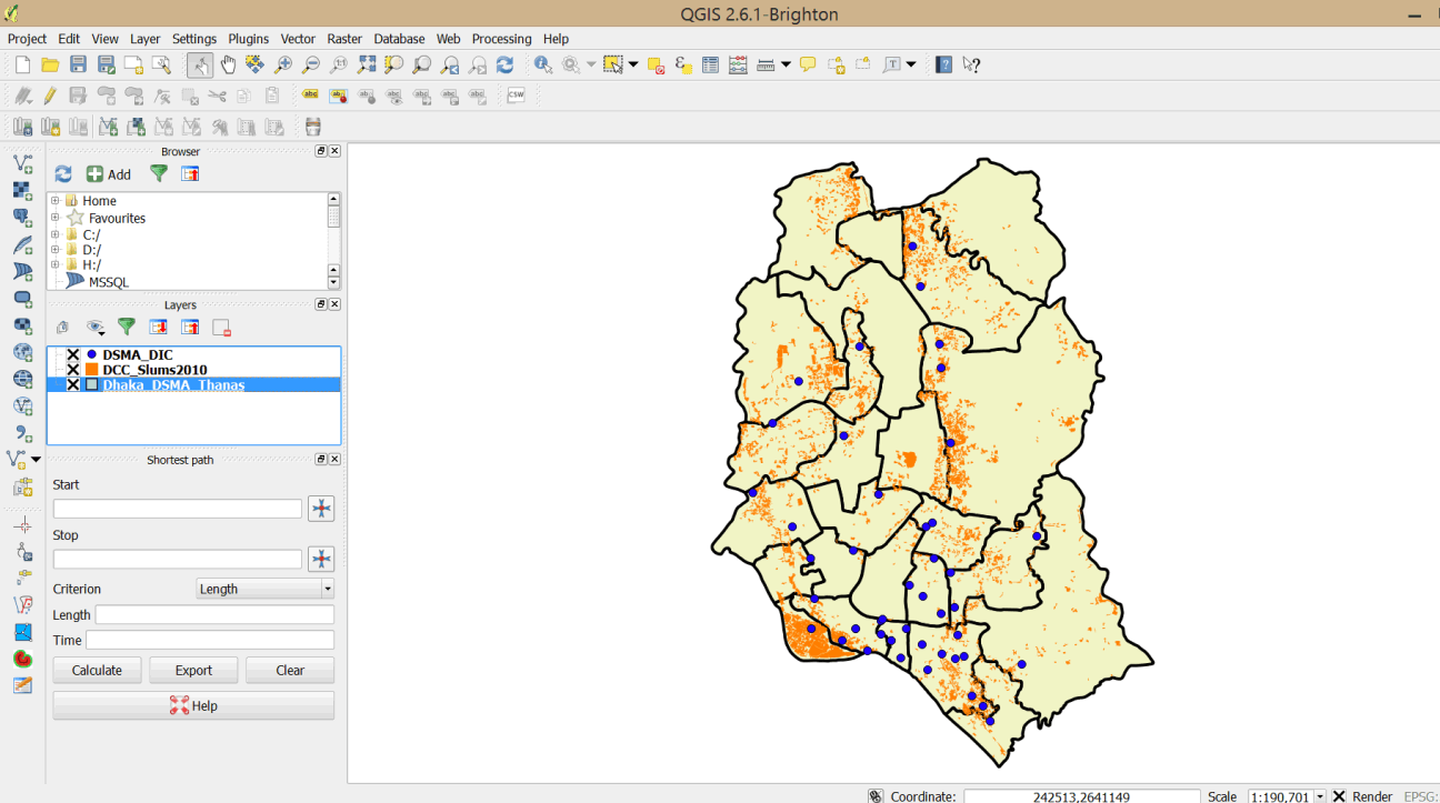
- Launch QGIS and start a new project. Save the project as Exercise 3e in MyExercises folder.
- Add the following vector layers from the exercise data folder – Dhaka_DSMA_Thanas.shp, DCC_Slums2010.shp and DSMA_DIC.shp.
3.5.3 Define DIC service areas (catchment areas)
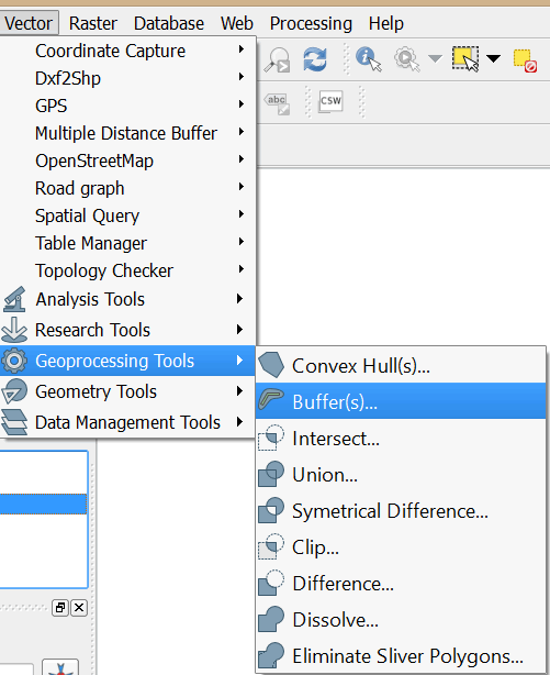
- On the main menu click on Vector > Geoprocessing Tools > Buffer(s)
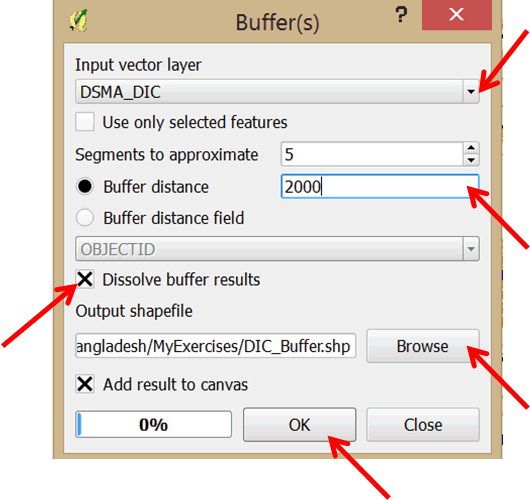
- In the dialog box that opens ensure that DSMA_DIC is the Input point vector layer. Set the Buffer distance to 2000 and select the Dissolve buffer results option.
- Browse to MyExercises folder and save the output shapefile as DIC_Buffer.shp. Click OK to run the tool.
- Close the dialog once the buffers are added to your map.
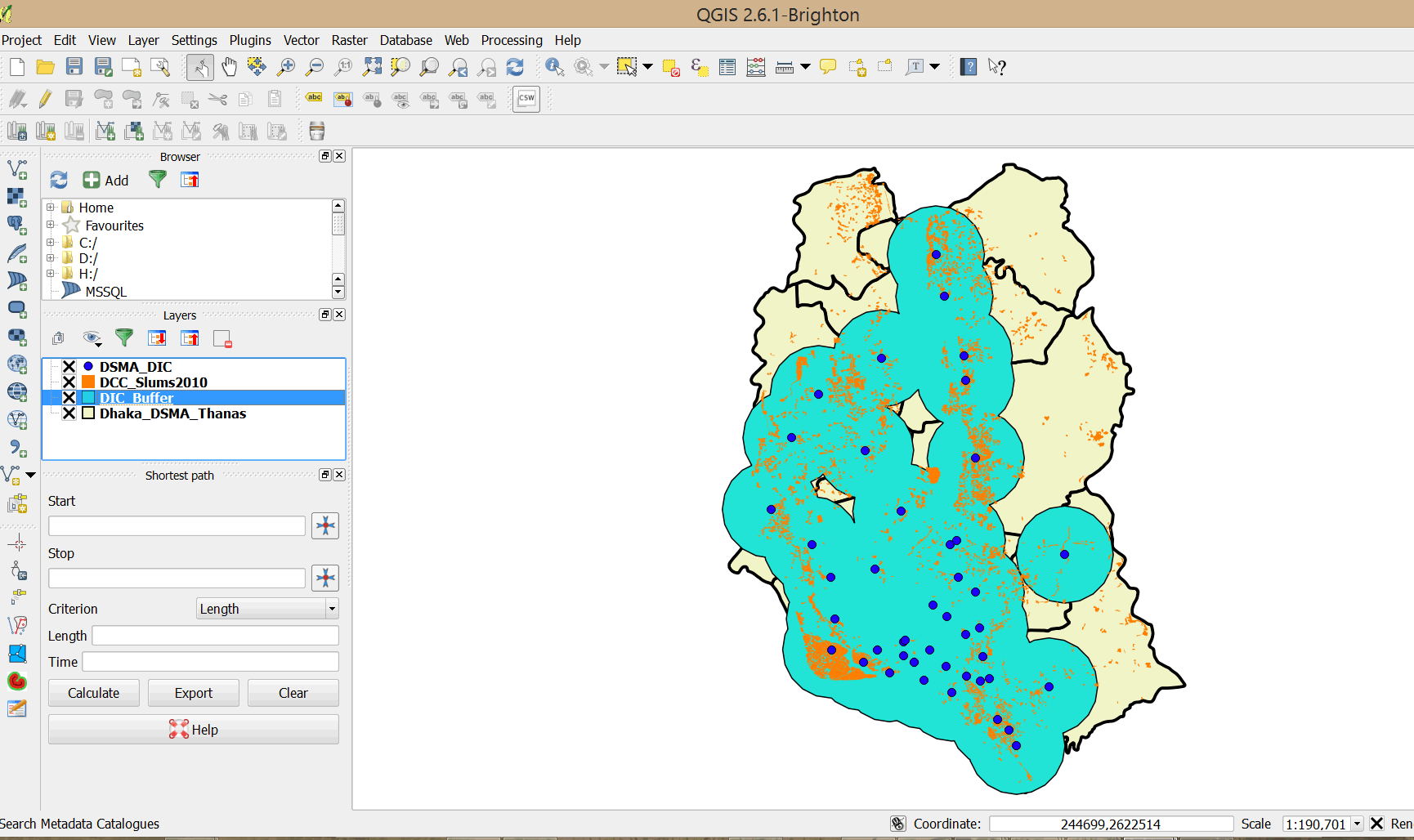
- Double-click on the DIC_Buffer layer and click Style. Change fill color to transparent and change the border color to red. Increase the border width to 0.460000.
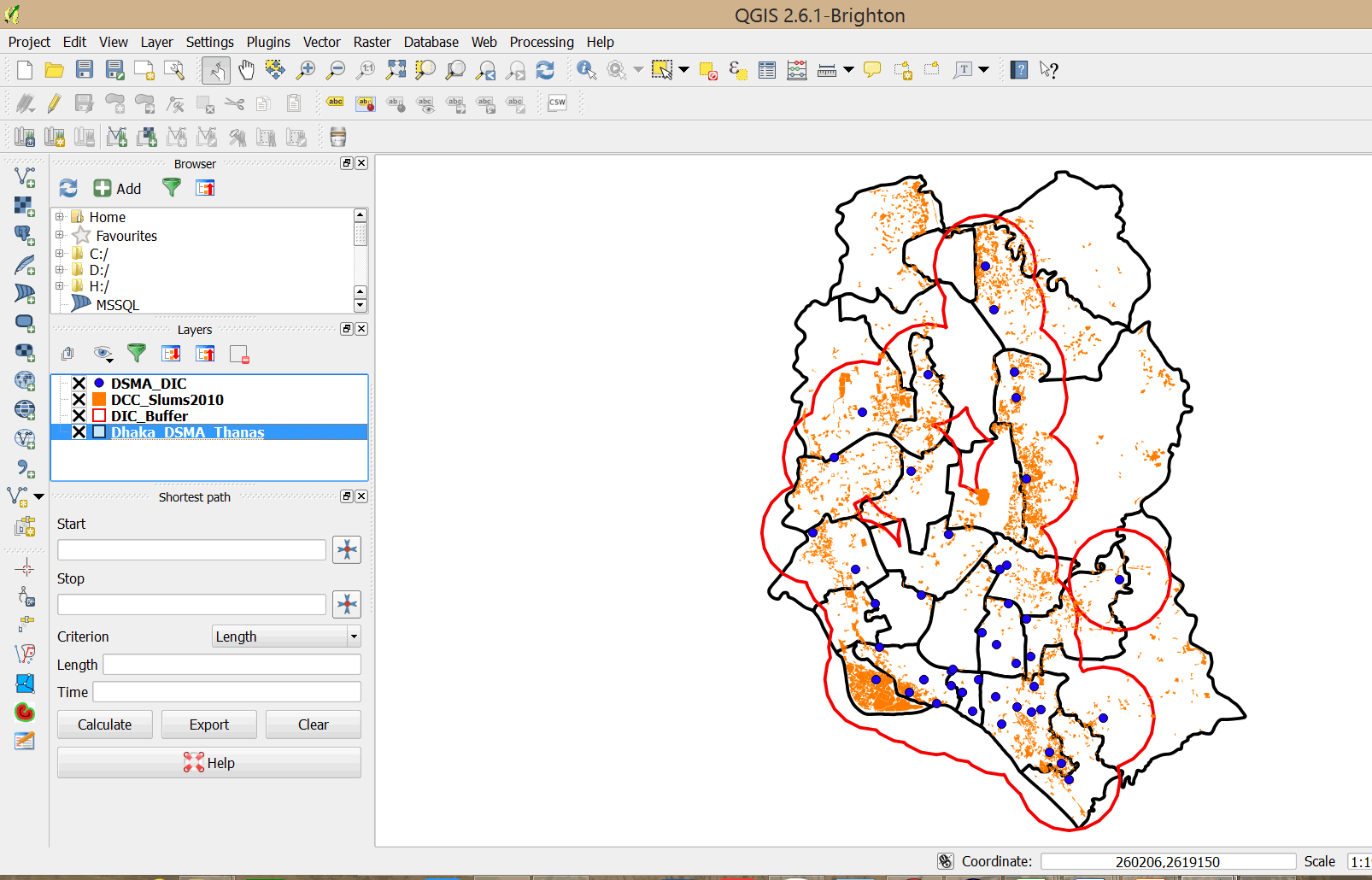
- This defines an area with a 2km radius around the drop in centers.
- Open the attribute table for DCC_Slums2010. The slums layer does not have any attributes on DIC.
- We shall now determine which slum dwellings are within the buffer area (catchment area). To do this we shall intersect the slum dwellings with the buffer layer using the Intersect tool.
3.5.4 Intersect features
Intersect is a geoprocessing function that overlays two themes and keeps only the polygons common to both.
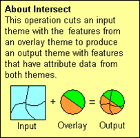
Source: ESRI
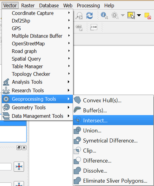
- On the main menu click on Vector > Geoprocessing Tools > Intersect
- In the dialog that opens select select DCC_Slums2010 as the Input vector layer. Select DIC_Buffer as the Intersect layer.
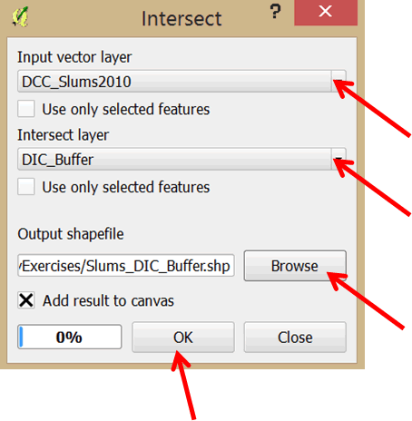
- Save the output shapefile in MyExercises folder as Slums_DIC_Buffer.
- Click OK
- A new layer of slum dwellings that fall within the buffer area is added to your map.
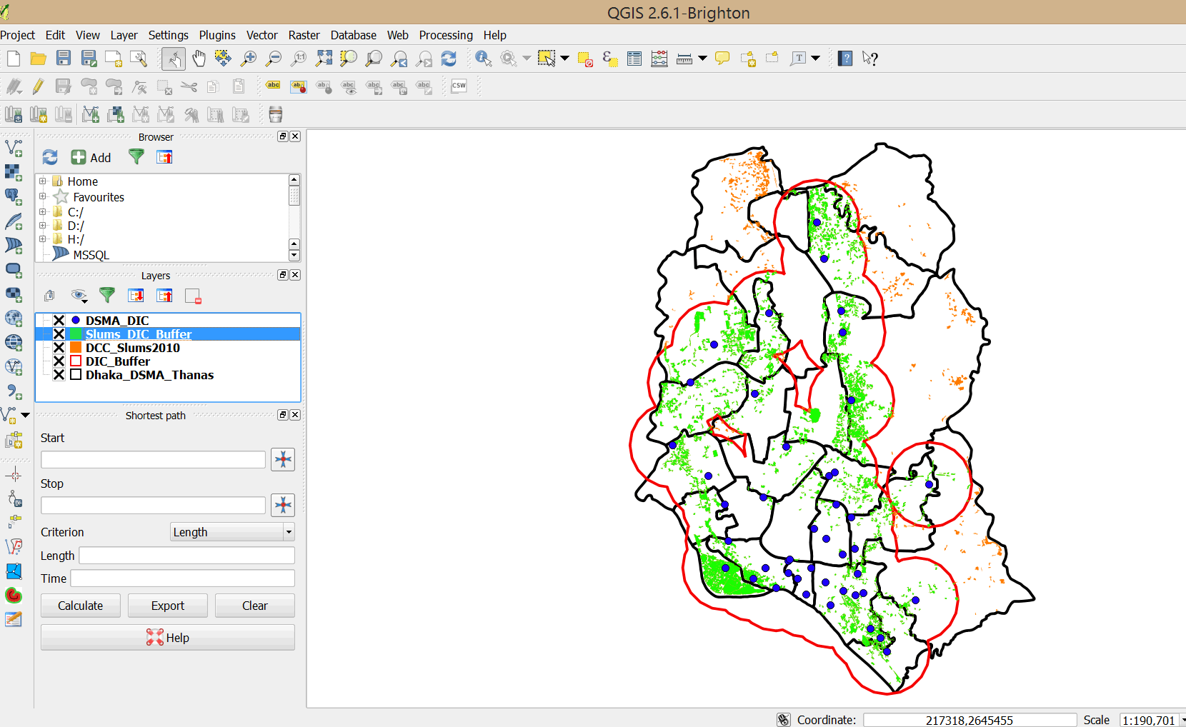
- Change the Slums_DIC_Buffer symbol properties to a transparent border. You can also change the fill color as appropriate.
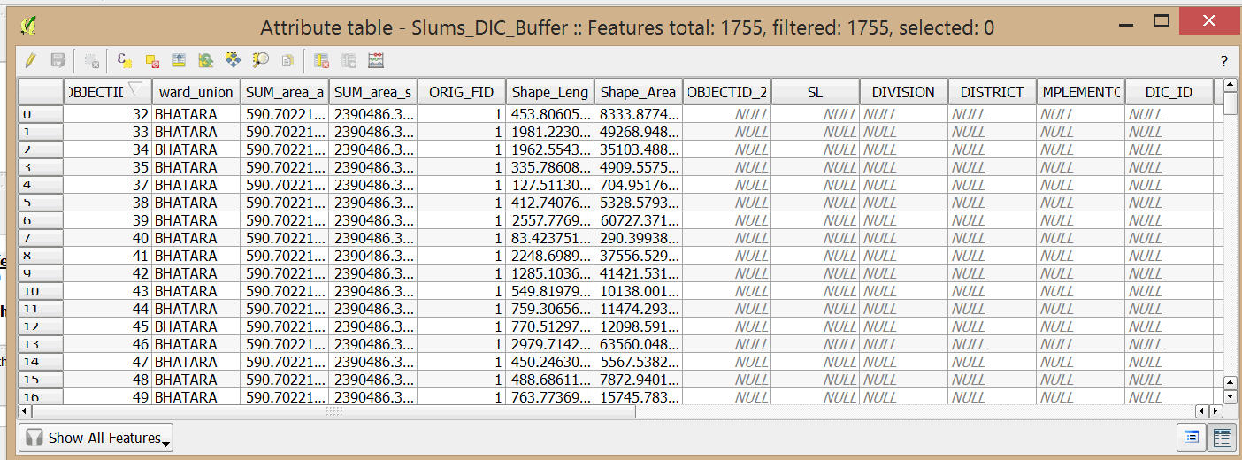
- Open the Attribute table of the Slums_DIC_Buffer. Unlike the thiessen polygons, the buffer tool does not define an area specific to each individual DIC. To do that you would have to do further analysis.
- Save your map to MyExercises folder.